Chapter 2 PMwG sampler and Signal Detection Theory
Here we demonstrate how to use the PMwG sampler package to run a simple signal detection theory (SDT) analysis on data from a lexical decision task. We recognise that it is unnecessary to use the sampler package for a simple analysis such as this; however, we hope this SDT example demonstrates the practicality of the PMwG sampler package.
2.0.1 Signal Detection Theory analysis of lexical decision task
We won’t cover SDT and lexical decision tasks (LDT) in detail here; however, we will explain how you can use the PMwG package with SDT in the context of a lexical decision task. If you require more information, please visit the SDT and LDT wikipedia pages. Also, this Frontiers in Psychology tutorial paper by Anderson (2015) is another good resource for SDT.
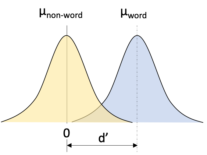
Figure 2.1: Simple SDT example of lexical decision task
The second parameter we denote is the criterion (C) parameter. The criterion is the point at which an individual responds non-word (to the left of C in Figure 2.2) or word (to the right of C in Figure 2.2) and it is set somewhere between the means of the two distributions. If you’re biased to respond word, the criterion would move to the left. Conversely, if you’re biased to respond non-word then the criterion would move to the right.
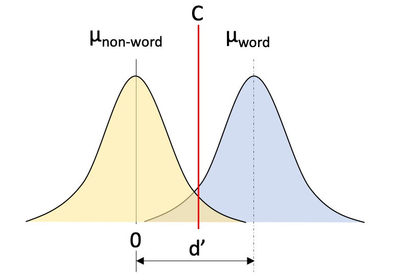
Figure 2.2: Simple SDT example of lexical decision task
2.0.2 The log-likelihood function
2.0.2.1 What is a log-likelhood?
The log-likelihood function is the ‘engine’ of the PMwG sampler. It is the way that the parameters of the model are connected to the data. In making this connection between data and parameters, the log-likelihood function actually defines the model and it’s associated psychological theory. The function takes in data (for a single subject) parameter values (for a single subject - ``random effects’’) and calculates the likelihood of the data given those random effect values. For most data sets, this process operates line-by-line: the log-likelihood is calculated for each observation and added. For example, we could compute the likelihood of a response time given a set of random effect values for a model. If the data are more likely given these random effect values are more likely (i.e. the model is closer to the data), the likelihood will be higher.
In the likelihood function, the parameter values must be assigned to the correct conditions and model parameters. For example, a linear regression model could have a slope and intercept parameter for easy and hard conditions i.e. four parameters. In this case, we would need to map the input parameter value for the slope in the easy condition onto the easy condition’s slope model parameter and then do the same for the hard slope and intercept parameters. This is much of the work of the log-likelihood function. Once mapped, we can use the appropriate values to calculate how likely were the data observed in each condition. Then we can calculate how likely the data are for the subject.
2.0.2.2 Writing a simple log-likelihood function
Let’s write a simple log-likelihood function for a fabricated data set. You can copy the code below to follow along with our example.
stim <- c("word", "word", "non-word", "word", "non-word", "non-word", "non-word", "word")
resp <- c("word", "word", "non-word", "word", "non-word", "non-word", "word", "non-word")
fab_data <- as.data.frame(cbind(stim, resp))
We create our dataset by combining a response resp and a stimulus stim vector into a data frame as shown in 2.1 below.
| stim | resp |
|---|---|
| word | word |
| word | word |
| non-word | non-word |
| word | word |
| non-word | non-word |
| non-word | non-word |
| non-word | word |
| word | non-word |
Our log-likelihood function will step through the data, line by line, and find a likelihood value for each trial, under two parameters; d-prime d and criterion C.
Here is our complete log-likelihood function. We have omitted some code from the code blocks below to enhance their appearance, so we encourage you to copy the log-likelihood function from the following code block if you’d like to follow along with our example. We’ll now step through each component of the log-likelihood below.
SDT_ll <- function(x, data, sample = FALSE){
  if (!sample) {
    out <- numeric(nrow(data))
    for (i in 1:nrow(data)) {
      if (stim[i] == "word") {
      if (resp[i] == "word") {
        out[i] <- pnorm(x["C"], mean = x["d"], sd = 1,
                        log.p = TRUE, lower.tail = FALSE)
      } else {
        out[i] <- pnorm(x["C"], mean = x["d"], sd = 1,
                        log.p = TRUE, lower.tail = TRUE)
      }
    } else {
      if (resp[i] == "word") {
        out[i] <- pnorm(x["C"], mean = 0, sd = 1,
                        log.p = TRUE, lower.tail = FALSE)
      } else {
        out[i] <- pnorm(x["C"], mean = 0, sd = 1,
                        log.p = TRUE, lower.tail = TRUE)
        }
      }
  }
  sum(out)
  }
}
We initialise the log-likelihood function with three arguments
xis a named parameter vector (e.g.pars)datais the datasetsample =sample values from the posterior distribution (For this simple example, we do not require asampleargument. )
The first if statement (line 2) checks if you want to sample, this is used for posterior predictive sampling which we will cover in later chapters. If you’re not sampling (like us in this example), you need to create an output vector out. The out vector will contain the log-likelihood value for each row/trial in your dataset.
From line 9, we check each row in the data set, first considering all trials with word stimuli if (stim[i] == "word" (line 10), and assign a likelihood for responding word (line 12-13) or non-word (line 15-16). The word distribution has a mean of x["d"] (d-prime parameter) and a decision criterion parameter x["C"]. If the response is word, we are considering values ABOVE or to the right of C in figure 2.2, so we set lower.tail = to FALSE. If the response is non-word, we look for values BELOW or to the left of C in figure 2.2 and we set lower.tail = to TRUE. The log.p = argument takes the log of all likelihood values when set to TRUE. We do this so we can sum all likelihoods at the end of the log-likelihood function.
  if (!sample) {
    for (i in 1:nrow(data)) {
      if (stim[i] == "word") {
        if (resp[i] == "word") {
          out[i] <- pnorm(x["C"], mean = x["d"], sd = 1,
                         log.p = TRUE, lower.tail = FALSE)
    } else {
      out[i] <- pnorm(x["C"], mean = x["d"], sd = 1,
                     log.p = TRUE, lower.tail = TRUE)
      }
From the else statement on line 18, we have the function for non-word trials i.e. stim[i] == "non-word". As can be seen below, the output value out[i] for these trials is arrived at in a similar manner to the word trials. We set the mean to 0 and the standard deviation sd to 1. If the response is word, we are considering values ABOVE or to the right of C in figure 2.2, so we set lower.tail = to FALSE. If the response is non-word, we look for values BELOW or to the left of C in figure 2.2 and we set lower.tail = to TRUE. Again we want the log of all likelihood values so we set log.p = TRUE.
else {
  if (resp[i] == "word") {
    out[i] <- pnorm(x["C"], mean = 0, sd = 1,
                    log.p = TRUE, lower.tail = FALSE)
        } else {
          out[i] <- pnorm(x["C"], mean = 0, sd = 1,
                         log.p = TRUE, lower.tail = TRUE)
        }
      }
The final line of code on line 24 sums the out vector and returns a log-likelihood value for your model.
2.1 Testing the SDT log-likelihood function
Before we run the log-likelihood function, we must create a parameter vector pars containing the same parameter names used in our log-likelihood function above i.e. we name the criterion C and d-prime parameter d. While we’re testing the log-likelihood, we assign arbitrary values to each parameter.
We can test run our log-likelihood function by passing the parameter vector pars and the fabricated dataset we created above fab_data.
## [1] -4.795029Now, if we change the parameter values, the log-likelihood value should also change.
## [1] -4.532791We can see the log-likelihood has changed. The second vector of parameter values are more likely than the first vector given the data.
2.2 SDT log-likelihood function for Wagenmakers experiment
Now that we’ve covered a simple test example, let’s create a log-likelihood function for the Wagenmakers et al. (2008) dataset.
2.2.1 Description of Wagenmakers experiment
If you’d like to follow our example, you will need to download the dataset from this link.The structure of the dataset will need to be modified in order to meet the requirements of the PMwG sampler. To do this, you can copy our script. You may attempt to modify the dataset yourself, but you must recreate the structure illustrated in table 2.2.
Participants were asked to indicate whether a letter string was a word or a non-word. A subset of Wagenmakers et al data are shown in table 2.2, with each line representing a single trial. We have a subject column with a subject id (1-19), a condition column cond which indicates the proportion of words to non-words presented within a block of trials. In word blocks (cond = w) participants completed 75% word and 25% non-word trials and for non-word (cond = nw) blocks 75% non-word and 25% word trials. The stim column lists the word’s frequency i.e. is the stimulus a very low frequency word (stim = vlf), a low frequency word (stim = lf), a high frequency word (stim = hf) or a non-word (stim = nw). The third column resp refers to the participant’s response i.e. the participant responded word (resp = W) or non-word (resp = NW). The two remaining columns list the response time (rt) and whether the paricipant made a correct (correct = 2) or incorrect (correct = 1) choice. For more details about the experiment please see the original paper.
| subject | condition | stim | resp | rt | correct |
|---|---|---|---|---|---|
| 1 | w | lf | W | 0.410 | 2 |
| 1 | w | hf | W | 0.426 | 2 |
| 1 | w | nw | NW | 0.499 | 2 |
| 1 | w | lf | W | 0.392 | 2 |
| 1 | w | vlf | W | 0.435 | 2 |
| 1 | w | hf | W | 0.376 | 2 |
| 1 | nw | lf | W | 0.861 | 2 |
| 1 | nw | hf | W | 0.563 | 2 |
| 1 | nw | nw | NW | 0.666 | 2 |
| 1 | nw | nw | NW | 1.561 | 2 |
| 1 | nw | nw | NW | 0.503 | 2 |
| 1 | nw | nw | NW | 0.445 | 2 |
Our log-likelihood function for Wagenmakers experimental data is similar to the function we wrote above, except now we require a criterion parameter for each condition and a d-prime parameter for each of the stim word types. This is illustrated in figure 2.3 below, where we have a non-word criterion Cnw, a word criterion Cw and three distributions for each of the stim types with corresponding d-prime for each distribution: dvlf, dlf, dhf.
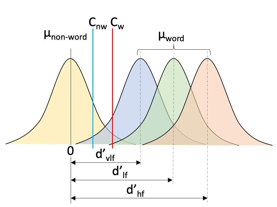
Figure 2.3: Signal detection theory example of lexical decision task
Here is our complete log-likelihood function for the Wagenmakers data set.
SDT_ll <- function(x, data, sample = FALSE){
  if (sample){
    data$response <- NA
  } else {
    out <- numeric(nrow(data))
  }
  if (!sample){
  for (i in 1:nrow(data)) {
    if (data$cond[i] == "w") {
    if (data$stim[i] == "hf") {
      if (data$resp[i] == "W") {
        out[i] <- pnorm(x["C.w"], mean = x["HF.d"], sd = 1,
                       log.p = TRUE, lower.tail = FALSE)
      } else {
        out[i] <- pnorm(x["C.w"], mean = x["HF.d"], sd = 1,
                       log.p = TRUE, lower.tail = TRUE)
      }
    } else if (data$stim[i] == "lf"){
      if (data$resp[i] == "W"){
        out[i] <- pnorm(x["C.w"], mean = x["LF.d"], sd = 1,
                       log.p = TRUE, lower.tail = FALSE)
      } else {
        out[i] <- pnorm(x["C.w"], mean = x["LF.d"], sd = 1,
                       log.p = TRUE, lower.tail = TRUE)
        }
      } else if (data$stim[i] == "vlf") {
        if (data$resp[i] == "W") {
          out[i] <- pnorm(x["C.w"], mean = x["VLF.d"], sd = 1,
                         log.p = TRUE, lower.tail = FALSE)
        } else {
          out[i] <- pnorm(x["C.w"], mean = x["VLF.d"], sd = 1,
                         log.p = TRUE, lower.tail = TRUE)
          }
        } else {
      if (data$resp[i] == "W") {
        out[i] <- pnorm(x["C.w"], mean = 0, sd = 1,
                       log.p = TRUE, lower.tail = FALSE)
      } else {
        out[i] <- pnorm(x["C.w"], mean = 0, sd = 1,
                       log.p = TRUE, lower.tail = TRUE)
        }
      }
    } else {
      if (data$stim[i] == "hf") {
        if (data$resp[i] == "W") {
          out[i] <- pnorm(x["C.nw"], mean = x["HF.d"], sd = 1,
                         log.p = TRUE, lower.tail = FALSE)
        } else {
          out[i] <- pnorm(x["C.nw"], mean = x["HF.d"], sd = 1,
                         log.p = TRUE, lower.tail = TRUE)
        }
      }  else if (data$stim[i] == "lf") {
        if (data$resp[i] == "W") {
          out[i] <- pnorm(x["C.nw"], mean = x["LF.d"], sd = 1,
                         log.p = TRUE, lower.tail = FALSE)
        } else {
          out[i] <- pnorm(x["C.nw"], mean = x["LF.d"], sd = 1,
                         log.p = TRUE, lower.tail = TRUE)
        }
      } else if (data$stim[i] == "vlf") {
        if (data$resp[i] == "W") {
          out[i] <- pnorm(x["C.nw"], mean = x["VLF.d"], sd = 1,
                         log.p = TRUE, lower.tail = FALSE)
        } else {
          out[i] <- pnorm(x["C.nw"], mean = x["VLF.d"], sd = 1,
                         log.p = TRUE, lower.tail = TRUE)
        }
      } else {
        if (data$resp[i] == "W") {
          out[i] <- pnorm(x["C.nw"], mean = 0, sd = 1,
                         log.p = TRUE, lower.tail = FALSE)
        } else {
          out[i] <- pnorm(x["C.nw"], mean = 0, sd = 1,
                         log.p = TRUE, lower.tail = TRUE)
        }
      }
    }
  }
  sum(out)
  }
}
Line 1 through to line 8 are the same as the log-likelihood we wrote for the fabricated dataset above. From line 9, we calculate the log-likelihood out[i] for word condition trials cond[i] == "w" when the stimulus is a high frequency word stim[i] == "hf" for each response. We do this by considering the upper tail of the high frequency word distribution lower.tail = FALSE, from the word criterion Cw, for word responses resp[i] == "W" and the lower tail for non-word responses (else statement on line 14). We then recycle this process for the remaining conditions/parameters in the experiment.
 if (data$cond[i] == "w") {
    if (data$stim[i] == "hf") {
      if (data$resp[i] == "W") {
        out[i] <- pnorm(x["C.w"], mean = x["HF.d"], sd = 1,
                       log.p = TRUE, lower.tail = FALSE)
      } else {
        out[i] <- pnorm(x["C.w"], mean = x["HF.d"], sd = 1,
                       log.p = TRUE, lower.tail = TRUE)
      }
This give us a log-likelihood for all data. Let’s test this…
pars <- log(c(C.w = 1, C.nw = 0.5, HF.d = 3, LF.d = 1.8, VLF.d = 0.7))
SDT_ll(pars, wgnmks2008, sample = FALSE)
## [1] -30801.712.2.2 Computation time of the log-likelihood function
You may have noticed that our log-likelihood function is slow and heavy on computer time when processing the data trial by trial. We recommend you write a ‘slow’ log-likelihood (as written above) to check it functions as it should before improving the function’s efficiency.
Now we’ll speed up our log-likelihood function. We have 16 possible values that could be assigned per line in the previous function (for the 16 cells of the design, given by proportion (2) x stimuli (4) x response (2)). Rather than looping over each trial, we could calculate the log-likelihood for each cell in the design and multiply the number of instances for each subject. To do this, we add a “n” column to the dataframe as shown in the code below.
wgnmks2008Fast <- as.data.frame(table(wgnmks2008$subject, wgnmks2008$cond,
                                  wgnmks2008$stim, wgnmks2008$resp))
names(wgnmks2008Fast) <- c("subject", "cond", "stim", "resp", "n")
Now our data frame looks like this..
| subject | cond | stim | resp | n |
|---|---|---|---|---|
| 1 | nw | hf | NW | 1 |
| 2 | nw | hf | NW | 2 |
| 3 | nw | hf | NW | 11 |
| 4 | nw | hf | NW | 0 |
| 5 | nw | hf | NW | 6 |
| 6 | nw | hf | NW | 9 |
For our SDT log-likelihood function, we add a multiplying factor (data$n[i]) to calculate the model log-likelihood and rather than looping over trials.
SDT_ll_fast <- function(x, data, sample = FALSE) {
  if (!sample) {
    out <- numeric(nrow(data))
    for (i in 1:nrow(data)) {
      if (data$cond[i] == "w") {
        if (data$stim[i] == "hf") {
          if (data$resp[i] == "W") {
            out[i] <- data$n[i] * pnorm(x["C.w"], mean = x["HF.d"],
                                     sd = 1, log.p = TRUE, lower.tail = FALSE)
          } else {
            out[i] <- data$n[i] * pnorm(x["C.w"], mean = x["HF.d"],
                                     sd = 1, log.p = TRUE, lower.tail = TRUE)
            }
          } else if (data$stim[i] == "lf") {
          if (data$resp[i] == "W") {
            out[i] <- data$n[i] * pnorm(x["C.w"], mean = x["LF.d"],
                                     sd = 1, log.p = TRUE, lower.tail = FALSE)
          } else {
            out[i] <- data$n[i] * pnorm(x["C.w"], mean = x["LF.d"],
                                     sd = 1, log.p = TRUE, lower.tail = TRUE)
          }
        } else if (data$stim[i] == "vlf") {
          if (data$resp[i] == "W") {
            out[i] <- data$n[i] * pnorm(x["C.w"], mean = x["VLF.d"],
                                     sd = 1, log.p = TRUE, lower.tail = FALSE)
          } else {
            out[i] <- data$n[i] * pnorm(x["C.w"], mean = x["VLF.d"],
                                     sd = 1, log.p = TRUE, lower.tail = TRUE)
          }
        } else {
          if (data$resp[i] == "W") {
            out[i] <- data$n[i] * pnorm(x["C.w"], mean = 0,
                                     sd = 1, log.p = TRUE, lower.tail = FALSE)
          } else {
            out[i] <- data$n[i] * pnorm(x["C.w"], mean = 0,
                                     sd = 1, log.p = TRUE, lower.tail = TRUE)
          }
        }
      }else{
        if (data$stim[i] == "hf") {
          if (data$resp[i] == "W") {
            out[i] <- data$n[i] * pnorm(x["C.nw"], mean = x["HF.d"],
                                     sd = 1, log.p = TRUE, lower.tail = FALSE)
          } else {
            out[i] <- data$n[i] * pnorm(x["C.nw"], mean = x["HF.d"],
                                     sd = 1, log.p = TRUE, lower.tail = TRUE)
          }
        }  else if (data$stim[i] == "lf"){
          if (data$resp[i] == "W") {
            out[i] <- data$n[i] * pnorm(x["C.nw"], mean = x["LF.d"],
                                     sd = 1, log.p = TRUE, lower.tail = FALSE)
          } else {
            out[i] <- data$n[i] * pnorm(x["C.nw"], mean = x["LF.d"],
                                     sd = 1, log.p = TRUE, lower.tail = TRUE)
          }
        } else if (data$stim[i] == "vlf") {
          if (data$resp[i] == "W") {
            out[i] <- data$n[i] * pnorm(x["C.nw"], mean = x["VLF.d"],
                                     sd = 1, log.p = TRUE, lower.tail = FALSE)
          } else {
            out[i] <- data$n[i] * pnorm(x["C.nw"], mean = x["VLF.d"],
                                     sd = 1, log.p = TRUE, lower.tail = TRUE)
          }
        } else {
          if (data$resp[i] == "W") {
            out[i] <- data$n[i] * pnorm(x["C.nw"], mean = 0,
                                     sd = 1, log.p = TRUE, lower.tail = FALSE)
          } else {
            out[i] <- data$n[i] * pnorm(x["C.nw"], mean = 0,
                                     sd = 1, log.p = TRUE, lower.tail = TRUE)
          }
        }
      }
    }
    sum(out)
  }
}
Now we have a fast(er) SDT log-likelihood function and we can compare its output with the slow log-likelihood function’s output to make sure it is functioning correctly.
pars <- log(c(C.w = 1, C.nw = 0.5, HF.d = 3, LF.d = 1.8, VLF.d = 0.7))
SDT_ll(pars, wgnmks2008, sample = FALSE)
## [1] -30801.71## [1] -30801.71Great—both functions produce the same log-likelihood! And we can run one final check by modifying the parameter vector’s values and seeing if the log-likelihood value updates.
pars <- log(c(C.w = 1, C.nw = 0.8, HF.d = 2.7, LF.d = 1.8, VLF.d = 1.3))
SDT_ll(pars, wgnmks2008, sample = FALSE)
## [1] -22168.95## [1] -22168.95As we saw with the fabricated dataset, the log-likelihood has changed. The second vector of parameter values are more likely than the first vector, given the data. We recommend speeding up your code however you wish. When you’re confident that your log-likelihood functions correctly, you should save it as a separate script so it can be sourced and loaded when running the sampler.
2.3 PMwG Framework
Now that we have written a log-likelihood function, we’re ready to use the PMwG sampler package.
Let’s begin by loading the PMwG package.
Now we require the parameter vector pars we specified above and a priors object called priors. The priors object is a list that contains two components:
theta_mu_meana vector that is the prior for the mean of the group-level mean parameterstheta_mu_vara covariance matrix that is the prior for the variance of the group-level mean parameters. In all examples we assume a diagonal matrix.
pars <- c("C.w", "C.nw", "HF.d", "LF.d", "VLF.d")
# This is the same as the `pars` vector specified above

priors <- list(
  theta_mu_mean = rep(0, length(pars)),
  theta_mu_var = diag(rep(1, length(pars)))
)
The priors object in our example is initiated with zeros. An important thing to note is that to facilitate Gibbs sampling from the multivariate normal distribution for the group parameters, the random effects must be estimated on the real line. In our SDT example, the parameters are free to vary along the real line so no transformation of the random effects is required. We expand on this point in more detail in later examples where parameters are bounded and require transformation. The prior on the covariance matrix is hard-coded as the marginally non-informative prior of Huang and Wand, as discussed in the PMwG paper.
The next step is to load your log-likelihood function/script.
Once you have set up your parameters, priors and written a log-likelihood function, the next step is to initialise the sampler object.
The pmwgs function takes a set of arguments (listed below) and returns a list containing the required components for performing the particle metropolis within Gibbs steps.
data =a data frame (e.g.wgnmks2008Fast) with a column for participants calledsubjectpars =the model parameters to be used (e.g.pars)prior =the priors to be used (e.g.priors)ll_func =name of log-likelihood function you’ve sourced above (e.g.SDT_ll_fast)
2.3.1 Model start points
You have the option to set model start points. We use 0 for the mean (mu) and a variance (sig2) of 0.01. If you chose not to specify start points, the sampler will randomly sample points from the prior distribution.
The start_points object contains two vectors:
mua vector of start points for the mean the model parameterssig2vector containing the start points of the covariance matrix of covariance between model parameters.
2.3.2 Running the sampler
Okay - now we are ready to run the sampler.
Here we are using the init function to generate initial start points for the random effects and storing them in the sampler object. First we pass the sampler object from above that includes our data, parameters, priors and log-likelihood function. If we decided to specify our own start points (as above), we would include the start_mu and start_sig arguments.
Now we can run the sampler using the run_stage function. The run_stage function takes four arguments:
xthesamplerobject including parameters that was created from the init function above.stage =the sampling stage (e.g."burn","adapt"or"sample")iter =is the number of iterations for the sampling stage. This is similar to running deMCMC, where it takes many iterations to reach the posterior space. Default = 1000.particles =is the number of particles generated on each iteration. Default = 1000.display_progress =shows progress bar for current stagen_cores =the number of cores to be used when running the samplerepsilon =is a value between 0 and 1 which reduces the size of the sampling space. We use lower values of epsilon when there are more parameters to estimate. Default = 1.
It is optional to include the iter = and particles = arguments. If these are not included, iter and particles default to 1000. The number of iterations you choose for your burn-in stage is similar to choices made when running deMCMC; however, this varies depending on the time the model takes to reach the ‘real’ posterior space.
First we run our burn-in stage by setting stage = to "burn".
burned <- run_stage(sampler,
                    stage = "burn",
                    iter = 1000,
                    particles = 20,
                    display_progress = TRUE,
                    n_cores = 8)
Now we run our adaptation stage by setting stage = "adapt". This function creates an efficient proposal distribution. The sampler will attempt to create the proposal distribution after 20 unique particles have been accepted for each subject. The sampler will then test whether the distribution was able to be created and if it was created, the sampler will move to the next stage otherwise the sampler will continue to sample. The number of iterations needs to be great enough to generate enough unique samples. The sampler will automatically exit the adapt stage when it has enough unique samples to create a multivariate normal ‘proposal’ distribution for each subject’s random effects. Thus we set iterations to a high number, as it should exit before reaching this point.
At the start of the sampled stage, the sampler object will create a ‘proposal’ distribution for each subject’s random effects using a conditional multi-variate normal. This proposal distribution is then used to efficiently generate new particles for each subject which means we can reduce the number of particles on each iteration whilst still achieving acceptance rates.
2.4 Check the sampling process
It is a good idea to check your samples by producing some simple plots as shown below. The first plot gives an indication of the trace for the group level parameters. In this example, you will see the chains take only several iterations before arriving at the posterior; however, this may not always be the case. Each parameter trace (horizontal lines on plot 2.4) should be stationary i.e. the trace should not trend up or down, and once the sampler reaches the posterior, the trace should remain relatively ‘thin’. If the trace is wide and bounces between large values (e.g. between -3 and 3) then there may be an error in your log-likelihood function.
As you can see in 2.4, the traces are clearly stable. Note that the number of iterations for the adaptation stage here is quite short because it’s easy to estimate and so gets lots of unique draws. Note: The sampling stages (i.e. burn-in, adapatation and sampling) are demarcated by the black, vertical lines.
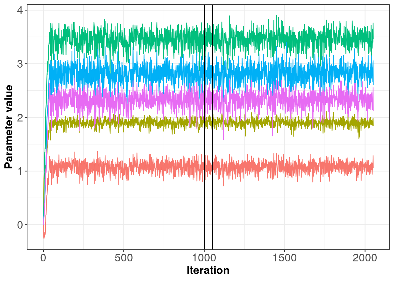
Figure 2.4: Posterior samples of parameters
The second plot below (figure 2.5) shows the likelihoods across iterations for each subject. Again we see that the likelihood values jump up after only a few iterations and then remain stable, with only slight movement.
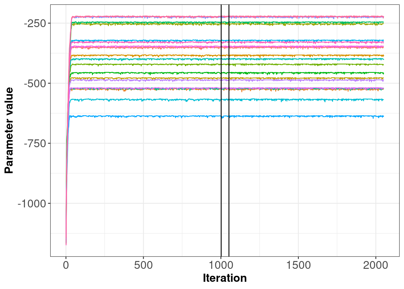
Figure 2.5: Posterior samples of subject log-likelihoods
2.5 Simulating posterior data
Now we’ll cover the sample operation within the fast log-likelihood function. We will use this on the full data set. The sample operation can be carried out in several ways (using rbinom etc). Please note that we do NOT recommend using this approach below and this should serve as an example only.
The sample process is similar to what we’ve covered above. We begin by assigning NAs to the response column to prepare it for simulated response data. We then consider a subset of the data, beginning with word condition and high-frequency hf word stimuli trials.
We then take the criterion for the word condition i.e. C.w. To simulate a response given our parameters we use rnorm to pick a random value from a normal distribution with mean = HF.d (i.e. high frequency word stimulus) and a SD of 1 and we test that value against the word criterion C.w. If the value is larger than C.w, the simulated response will be word otherwise, the simulated response will be non-word.
We repeat this process for each condition and stimulus combination as shown in the code block below.
{ else if (data$stim[i] == "lf") {
  data$resp[i] <- ifelse(test = (rnorm(1,
                                       mean = x["LF.d"],
                                       sd = 1)) > x["C.w"], "word", "non-word")
  } else if (data$stim[i] == "vlf") {
    data$resp[i] <- ifelse(test = (rnorm(1,
                                         mean = x["VLF.d"],
                                         sd = 1)) > x["C.w"], "word", "non-word")
    } else {
      data$resp[i] <- ifelse(test = (rnorm(1,
                                           mean = 0,
                                           sd = 1)) > x["C.w"], "word", "non-word")
      }
} else {
  if (data$stim[i] == "hf") {
    data$resp[i] <- ifelse(test = (rnorm(1,
                                         mean = x["HF.d"],
                                         sd = 1)) > x["C.nw"], "word", "non-word")
    } else if (data$stim[i] == "lf") {
          data$resp[i] <- ifelse(test = (rnorm(1,
                                               mean = x["LF.d"],
                                               sd = 1)) > x["C.nw"], "word", "non-word")
        } else if (data$stim[i] == "vlf") {
          data$resp[i] <- ifelse(test = (rnorm(1,
                                               mean = x["VLF.d"],
                                               sd = 1)) > x["C.nw"], "word", "non-word")
        } else {
          data$resp[i] <- ifelse(test = (rnorm(1,
                                               mean = 0,
                                               sd = 1)) > x["C.nw"], "word", "non-word")
          }
        }
Now we can run our simulation. Below is some code to achieve this.
n.posterior <- 20 # Number of samples from posterior distribution for each parameter.
pp.data <- list()
S <- unique(wgnmks2008$subject)
data <- split(x = wgnmks2008,
              f = wgnmks2008$subject)
for (s in S) {
  cat(s," ")
  iterations = round(seq(from = 1051,
                         to = sampled$samples$idx,
                         length.out = n.posterior))
  for (i in 1:length(iterations)) {
    x <- sampled$samples$alpha[, s, iterations[i]]
    names(x) <- pars
    tmp <- SDT_ll_fast(x = x,
                       data = wgnmks2008[wgnmks2008$subject == s,],
                       sample = TRUE)
    if (i == 1) {
      pp.data[[s]] <- cbind(i,tmp)
    } else {
      pp.data[[s]] <- rbind(pp.data[[s]], cbind(i, tmp))
    }
  }
}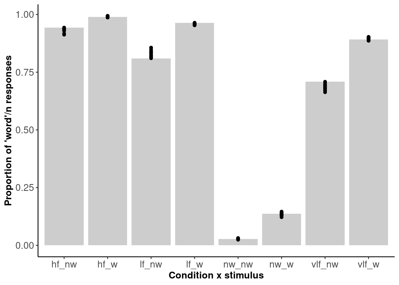
Figure 2.6: The proportion of ‘word’ responses within each cell of the design.
Figure 2.6 shows 20 posterior draws (dots) plotted against the data (bars). The posterior draws are for each individual subject - shown here is the average proportion of word responses. We can see that the model fits the data well.
References
Anderson, Nicole D. 2015. “Teaching Signal Detection Theory with Pseudoscience.” Frontiers in Psychology 6: 762.
Wagenmakers, Eric-Jan, Roger Ratcliff, Pablo Gomez, and Gail McKoon. 2008. “A Diffusion Model Account of Criterion Shifts in the Lexical Decision Task.” Journal of Memory and Language 58 (1): 140–59.